![]()
![]()
The data set used in this example is available in the example database installed with the software (called "DOE11_examples.rsgz11"). To access this database file, choose File > Help, click Open Examples Folder, then browse for the file in the DOE sub-folder.
The name of the example project is "Factorial - Taguchi OA Design Example."
Taguchi orthogonal array (OA) designs are often used in design experiments with factors that include more than two levels. Taguchi OA can be thought of as a general fractional factorial design.
Consider an experiment to study the effect of four three-level factors on a fine gold wire bonding process in an IC chip-package.* Taguchi OA L27 (3^13) is applied to identify the critical parameters in the wire bonding process. The response is the ball size. The smaller the ball size, the better the process.
For this example, the four factors and their associated levels are:
|
Factor |
Level 1 |
Level 2 |
Level 3 |
|
Force |
5 |
10 |
15 |
|
Power |
40 |
50 |
60 |
|
Time |
15 |
20 |
25 |
|
Temperature |
155 |
160 |
165 |
The experimenters create a Taguchi OA design folio, perform the experiment according to the design, and then enter the response values for further analysis. The design matrix and the response data are given in the "Taguchi OA L27(3^13)" folio. The following steps describe how to create this folio on your own.
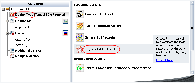
Choose Insert > Designs > Standard Design to add a standard design folio to the current project.
![]()
Click Design Type in the folio's navigation panel, and then select Taguchi OA Factorial in the input panel.
Rename the response by clicking Response 1 in the navigation panel and entering Ball Size for the Name in the input panel.
Specify the number of factors by clicking the Factors heading in the navigation panel and choosing 4 from the Number of Factors drop-down list.
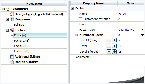
Define each factor by clicking it in the navigation panel and editing its properties in the input panel. The properties are given in the table above. The first factor is defined as shown next. (Note that every factor must be configured to have three levels.)
Rename the folio by clicking the Experiment1 heading in the navigation panel and entering Taguchi OA L27 (3^13) for the Name in the input panel.
Click the Additional Settings heading to choose an orthogonal array and assign factors to columns in the array.
In the input panel, choose L27 (3^13) from the Taguchi Design Type drop-down list. This specifies the orthogonal array that will be used to generate the design.
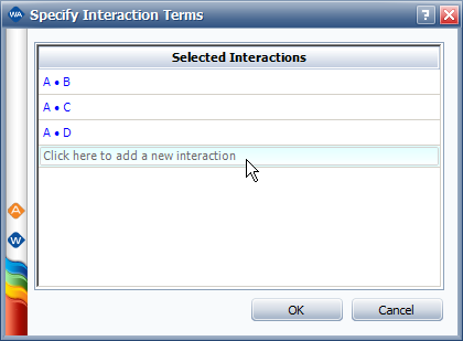
To have the software determine which columns in the array will be assigned to the factors, click the Specify Interaction Terms link. In the window that appears, enter all possible two-way interactions between the factors being investigated. The easiest way to do this is by repeatedly clicking the row that says "Click here to add a new interaction" until the row disappears.
Click OK to close the window. Force is now assigned to column 1 of the array, Power to 2, Time to 5 and Temperature to 9, as shown next.
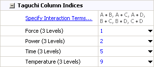
These column assignments will be used to generate a design that does not alias any of the two-way interactions you entered in the Specify Interaction Terms window with any main effects.
Finally, click the Build icon on the control panel to create a Data tab that allows you to view the test plan and enter response data.
![]()
The data set for this example is given in the "Taguchi OA L27 (3^13)" folio of the example project. After you enter the data from the example folio, you can perform the analysis by doing the following:
Note: To minimize the effect of unknown nuisance factors, the run order is randomly generated when you create the design. Therefore, if you followed these steps to create your own folio, the order of runs on the Data tab may be different from that of the folio in the example file. This can lead to different results. To ensure that you get the very same results described next, show the Standard Order column in your folio, then click a cell in that column and choose Sheet > Sheet Actions > Sort > Sort Ascending. This will make the order of runs in your folio the same as that of the example file. Then copy the response data from the example file and paste it into the Data tab of your folio.
On the Analysis Settings page of the control panel, select to use Individual Terms in the analysis.
Return to the Main page of the control panel and click the Calculate icon.
![]()
Click the View Analysis Summary icon on the control panel and select to the view the ANOVA Table.
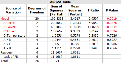
From this table, you can see that effects A, B, C are significant. To simply the analysis, the next step is to recreate the model using only the significant terms.
The results for the reduced model are given in the "Reduced Model" folio of the example project. The following steps describe how to create this folio on your own and then use the results to find the factor settings that provide the smallest deviation in height.
Right-click the design folio in the current project explorer and select Duplicate Item from the shortcut menu. Rename the new folio with an appropriate name.
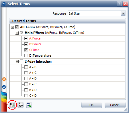
Click the Select Terms icon on the new folio's control panel.
![]()
In the Select Terms window that appears, click the Select Significant Effects button to select only the significant effects to calculate the new model, as shown next, then click OK.
Click the Calculate icon in the new folio's control panel.
Click the View Analysis Summary icon on the control panel. In the Analysis Summary window that appears, view the Diagnostic Information table. The table is shown next. In order to identify which factor settings can provide the smallest ball size (and hence the best process), look for the runs in the table with the Fitted Value (YF) closest to zero (highlighted).
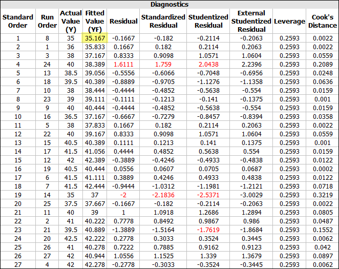
You can see that the first run in the standard order (8th run in the run order) is at the best combination of settings. The settings for this particular run on the Data tab is shown to be A = 5, B = 40, C = 15. Under these settings, the expected ball size is lowest.
Note that the best factor settings in this case are limited to those settings actually used in the experiment. This limitation can be avoided using response surface methodology, which may allow you to find the optimal settings for the manufacturing process.
* T. Hou, S. Chen, T. Lin and K. Huang, "An integrated system for setting the optimal parameters in IC chip-package wire bonding process," Int. J Adv Manuf Technology, 2006, 30, 247-253.
** G. Taguchi, S. Chowdhury and Y. Wu, Taguchi's Quality Handbook, Hoboken, New Jersey, Wiley, 2004.
© 1992-2017. HBM Prenscia Inc. ALL RIGHTS RESERVED.
 |
E-mail Link |