	Related Topics and Links:
	General Full Factorial Designs

General Full Factorial Designs: Example

The data set used in this example is available in the example database installed with the software (called "DOE11_examples.rsgz11"). To access this database file, choose File > Help, click Open Examples Folder, then browse for the file in the DOE sub-folder.

The name of the example project is "Factorial - General Full Factorial Design."

In this example, a soft drink bottler is interested in obtaining more uniform fill heights in the bottles (as described in Montgomery, D. C. Design and Analysis of Experiments, 5th edition, John Wiley & Sons, New York, 2001). The filling machine is designed to fill each bottle to the correct target height, but in practice, there is variation around this target, and the bottler would like to examine the sources of this variability so she can reduce it. There are three control factors. The factors and associated levels that will be used in the experiment are shown next.

Factor	Unit	Level 1	Level 2	Level 3
Percent Carbonation	%	10	12	14
Operating Pressure	psi	25	30	-
Line Speed	bpm	200	250	-

There are two replicates at each factor setting, making a total of 24 runs. The response is the average deviation from the target fill height observed in a production run of bottles. Positive deviations are fill heights above the target.

Design the Experiment

The experimenters create a general full factorial design, perform the experiment according to the design, and then enter the response values into the folio for analysis. The design matrix and the response data are given in the "Soft Drink Bottling Experiment" folio. The following steps describe how to create this folio on your own.

Choose Insert > Designs > Standard Design to add a standard design folio to the current project.

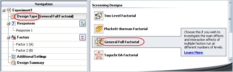
Click Design Type in the folio's navigation panel, and then select General Full Factorial in the input panel.

Rename the response by clicking Response 1 in the navigation panel and entering Height Deviation in the input panel.

Specify the number of factors by clicking the Factors heading in the navigation panel and choosing 3 from the Number of Factors drop-down list.
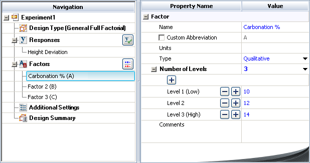
Define each factor by clicking it in the navigation panel and editing its properties in the input panel. The properties are given in the table above. The first factor is defined as shown next.

Rename the folio clicking the Experiment1 heading in the navigation panel and entering Soft Drink Bottling Experiment for the Name in the input panel.
Click the Additional Settings heading. In the input panel, set the number of Replicates to 2.
Finally, click the Build icon on the control panel to create a Data tab that allows you to view the test plan and enter response data.

Analysis and Results - Part 1

The data set for this example is given in the "Soft Drink Bottling Experiment" folio of the example project. After you enter the data from the example folio, you can perform the analysis by doing the following:

Note: To minimize the effect of unknown nuisance factors, the run order is randomly generated when you create the design. Therefore, if you followed these steps to create your own folio, the order of runs on the Data tab may be different from that of the folio in the example file. This can lead to different results. To ensure that you get the very same results described next, show the Standard Order column in your folio, then click a cell in that column and choose Sheet > Sheet Actions > Sort > Sort Ascending. This will make the order of runs in your folio the same as that of the example file. Then copy the response data from the example file and paste it into the Data tab of your folio.

On the Analysis Settings page of the control panel, select to use Individual Terms in the analysis.
Return to the Main page of the control panel and click the Calculate icon.

Click the View Analysis Summary icon on the control panel and select to the view the ANOVA Table.

From this table, you can see that effects A, B, C and AB are significant. To simplify the analysis, the next step is to recreate the model using only the significant terms.

Analysis and Results - Part 2

The results for the reduced model are given in the "Reduced Model" folio of the example project. The following steps describe how to create this folio on your own and then use the results to find the factor settings that provide the smallest deviation in height.

Right-click the design folio in the current project explorer and select Duplicate Item from the shortcut menu. Rename the new folio with an appropriate name.
Click the Select Terms icon on the new folio's control panel.

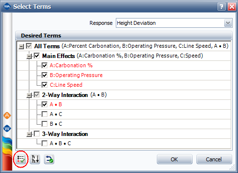
In the Select Terms window that appears, click the Select Significant Effects button to select only the significant effects to calculate the new model, as shown next, then click OK.

Click the Calculate icon in the new folio's control panel.

Click the View Analysis Summary icon on the control panel. In the Analysis Summary window that appears, view the Diagnostic Information table. The table is shown next. In order to identify which factor settings can provide the smallest height deviation, look for the runs in the table with the Fitted Value (YF) closest to zero (highlighted).

Conclusions

You can see that the 9th and 10th runs in the standard order are at the best combination of settings. The settings for these particular runs on the Data tab are shown to be A = 12, B = 25, C = 200. Under these settings, the expected deviation is lowest.

Note that the best factor settings in this case are limited to those settings actually used in the experiment. This limitation can be avoided using response surface methodology, which may allow you to find the optimal settings for the manufacturing process.

E-mail Link