Times-to-Failure Data from Multiple Systems

The multiple systems data types are for analyzing failure times from multiple identical systems (where the data set from each system is identified by the specific System ID). In multiple systems analysis, RGA combines the operating hours of the systems to create a single equivalent system, which allows you to evaluate all the failures and fixes that occurred during testing. The parameters of the equivalent system, along with the results of the goodness-of-fit tests for that system, are calculated automatically when you analyze the data sheet. Any plots generated for the data set and analyses via the Quick Calculation Pad will be also based on the equivalent system.

There is a choice of four data sheets depending on how the operating times of the systems are determined:

In all these data sheets, the operating time of the failed system is recorded for each failure. The following table summarizes how these data sheets obtain or estimate the operating times of the other non-failed systems.

If you will assume that when failures are found the same set of fixes is applied to all of the systems at the same time (traditional reliability growth analysis), then you can use the Crow-AMSAA (NHPP) or Duane models. Once the fix has been implemented for all systems, the test is resumed; therefore, each row in the data sheet will represent a different design configuration.

If you want to account for different fix strategies used for different failure modes (growth projections analysis), choose the Crow Extended model. You will be required to identify and classify the failure mode responsible for each failure (i.e., A = no fix, BC = fixed during test or BD = delayed fix), as well as specify the effectiveness factor for each delayed fix.

When you select the Crow Extended model, the Classification and Mode columns will be inserted into the data sheet. You can also manually insert or remove these columns by choosing Growth Data > Format & View > [Insert Columns/Delete Columns] > Projections. The Crow Extended model and mode classifications are discussed in Failure Mode Classifications.

By default, all data sheets include a Comments column for logging any pertinent information about each row of data. You can add a second comments column or delete the columns by choosing Growth Data > Format & View > [Insert Columns/Delete Columns] > Comments. The information in these columns does not affect the calculations in the folio.

Multiple Systems - Known Operating Times

The Known Operating Times data type is used for situations when multiple identical systems are tested and the exact operating times for all systems are known. When a failure occurs in any of the systems, the exact operating times for all systems (both failed and non-failed) are recorded. The analysis assumes that the fixes are applied to all of the systems at the same time so they continue to have the same configuration.

The Time System [x] columns are for recording the failure times/operating times of the units. The times can be cumulative (where each row shows the total amount of time when the failure occurred) or non-cumulative (where each row shows the incremental time from when the last failure occurred). (See Cumulative vs. Non-Cumulative Data.) By default, the data sheet is configured for two systems. To insert or remove additional columns, choose Growth Data > Format & View > [Insert Columns/Delete Columns] > System/Unit.

The Failed System ID column is for recording the ID number of the system that failed. It must be represented by a positive integer.

The following data sheet shows an example in which the times are cumulative. The first failure occurred for System 1 (indicated by a 1 in the first column for row 1). At that point, the operating times for both systems were recorded — 7 hours for System 1 and 10 hours for System 2 — and the same fix was applied on both systems. The next failure occurred for System 2 (indicated by a 2 in the first column for row 2). Once again, the operating times for both systems were recorded — 15 hours for System 1 (8 since the last event) and 17 hours for System 2 (7 since the last event). The rest of the data can be interpreted in a similar manner.

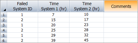
Multiple Systems - Known Operating Times Data Sheet for
Traditional Reliability Growth Analysis (Cumulative)

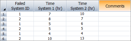
Multiple Systems - Known Operating Times Data Sheet for
Traditional Reliability Growth Analysis (Non-Cumulative)

Multiple Systems - Concurrent Operating Times

The Concurrent Operating Times data type is used for situations when multiple identical systems are tested but a system’s exact operating time can be known only when it fails. The analysis assumes that the systems all began with the same configuration, they operate concurrently, they accumulate usage at the same rate and they receive fixes at the same time. Therefore, when a failure occurs in any of the systems, the exact operating time for the failed system is recorded and this time is also used as the operating times for the other non-failed systems.

With this data type, you can enter the data in the Normal View or Advanced Systems View. The following example shows the Normal View. The System ID column is for recording the ID of the system that the data point relates to. The Event column specifies whether the row represents the start time (S), failure time (F) or end time (E) of the system. The Time to Event column is for recording the total cumulative test time when the specified event occurred.

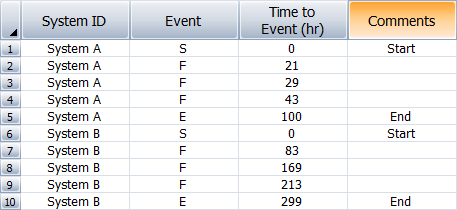
Multiple Systems - Concurrent Operating Times Data Sheet (Normal View)
for Traditional Reliability Growth Analysis

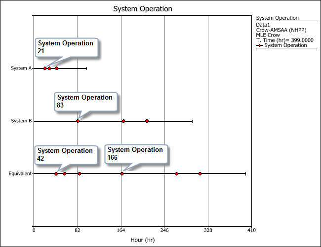
The following plot shows the failure times of both systems in the example, along with the timeline for their equivalent system. When the first failure occurred at 21 hours (System A), the total operating time for the test (represented by the equivalent system) is 42 hours because there are two systems running concurrently. In other words, the analysis multiplies the failure time of the failed system by the total number of systems in the test to obtain the equivalent operating time. Similarly, the first failure of System B (at 83 hours) is shown in the equivalent system as occurring at 166 hours.

Multiple Systems with Dates

Like the Concurrent Operating Times data type, the Multiple Systems with Dates data type is used for situations when multiple identical systems are tested but a system’s exact operating time can be known only when it fails. However, this data type can be used when the systems did not all begin with the same configuration and/or they are not operated concurrently (although it still assumes that the fixes are applied to all of the systems at the same time). When a failure occurs in any of the systems, the exact operating time for the failed system is recorded and the software estimates the operating times for the other non-failed systems using the exact calendar dates recorded for all events. Specifically, the software uses the dates to calculate the average daily usage rate of each non-failed system over the relevant time period.

The data sheet is the same as the Concurrent Operating Times data sheet but with a Date column for recording the calendar date of the events. You can enter the data in the Normal View or Advanced Systems View. The following example shows a data set in the Normal View.

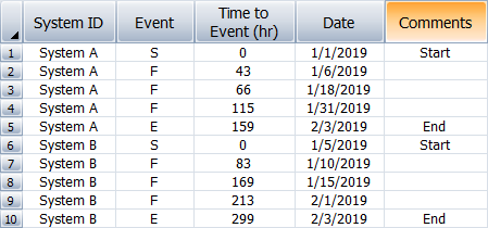
Multiple Systems with Dates Data Sheet (Normal View)
for Traditional Reliability Growth Analysis

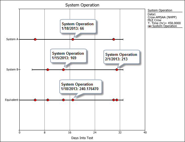
The following plot shows the failure times of both systems in the example, along with the timeline for their equivalent system. For example, the plot shows that when System A failed on 1/18/2019, it had accumulated 66 hours of operating time, but we don’t know the exact operating time for System B at that point.

We do know that when System B failed on 1/15/2019 it had accumulated 169 hours of test time and then when it failed again on 2/1/2019, it had accumulated 213 hours. The total accumulated test time of System B between these two periods is 213-169=44 hours.

If we divide this result by the number of days (17), we obtain the average daily usage rate of System B during that period (2.588235 hours/day).

This can then be used to estimate the number of hours System B accumulated in the 2 days between the first failure of System B on 1/15/2019 and the first failure of System A on 1/18/2019 (2 x 2.5882 = 5.176470 hours).

Therefore, the analysis assumes that the operating time of System B was 174.176470 hours when System A failed on 1/18/2019.

For the equivalent system, the estimated operating time on 1/18/2019 is the summation of the observed operating time for System A and the estimated operating time for System B, which is 240.176470 hours.

Multiple Systems with Event Codes

The Multiple Systems with Event Codes data type is similar to the Concurrent Operating Times data type except that it always requires you to identify and classify the failure mode responsible for each failure (see Failure Mode Classifications). It also allows you to use codes to identify other types of events besides failures (e.g., the time when a fix was implemented for a particular failure mode, performance or quality issues that can be included or excluded from the analysis, etc.). This data type can be used when fixes are not implemented simultaneously for all systems. The Crow Extended model is used for the analysis.

With this data type, you can enter the data in the Normal View or Advanced Systems View. The following example shows the Normal View. The Classification and Mode columns are for identifying and classifying the failure mode responsible for each failure. The Event column specifies the type of event the data point represents. See Event Codes for Crow Extended for information on all five possible event types. In the following data sheet, S = start time, F = failure time, I = the time when the fix for a particular failure mode was implemented, P = performance failure, Q = quality failure and E = end time.

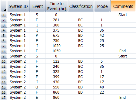
Multiple Systems with Event Codes Data Sheet (Normal View)
for Reliability Growth Projections Analysis

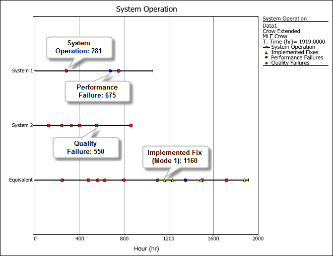
In this case, the process of combining the data set for the equivalent system is the same as described above for the Concurrent Operating Times data sheet, but with the addition of taking into account the time of implemented fixes across different systems. The implemented fix time is obtained by computing for the total time that the system spent in the same design configuration for a particular mode before the implemented fix took place. For these plots, the different types of events are shown in different colors: failure (red circle), implemented fix (yellow triangle), performance failure (blue circle) and quality failure (green diamond).

E-mail Link

Data Type	Operating Times of Non-Failed Systems	All systems must operate at same rate?	All systems must start the test at the same time?
Known Operating Times	User provides the exact operating times for both failed system and all other non-failed systems.	No
Concurrent Operating Times	RGA uses the failure time of the failed system as the operating times of the non-failed systems.	Yes
Multiple Systems with Dates	RGA uses calendar dates to estimate the operating times of non-failed systems based on their average daily usage rate for the relevant time period.	No
Multiple Systems with Event Codes	Same as "Concurrent Operating Times."	Yes