Gap Analysis

Gap analysis is used in situations where issues such as oversight, biases, human error, technical difficulties, etc. cause some portion of the data to be erroneous or completely missing. This causes the analysis to return distorted estimates of the growth rate and actual system reliability. In this type of situation, you can use the Gap Analysis feature in RGA to analyze the data set.

Gap analysis assumes that the information within the problematic time interval is unavailable or unreliable and does not use any entries that have been made for that time period. Instead, the number of failures for that interval is assumed to be unknown, but the rest of the data follow the Crow-AMSAA model. The analysis retains the contribution of the interval to the total test time, but no assumptions are made regarding the actual number of failures over the interval.

This analysis is available when you use the Failure Times data type with the Crow-AMSAA (NHPP) model using standard calculations (gap intervals are not compatible with Change of Slope calculations). You can define one gap interval per data set. Each gap is a time range that exists within the data, and it has a defined start time and end time. There must be at least one failure before and after the specified gap interval.

Example

The data set used in this example is available in the example database installed with the software (called "RGA19_Examples.rsgz19"). To access this database file, choose File > Help, click Open Examples Folder, then browse for the file in the RGA sub-folder.

A system is put through a reliability growth testing program. The test is terminated after 1,000 hours of testing, and a total of 86 failures were observed during that period. The data are recorded in a Failure Times data sheet and analyzed with the Crow-AMSAA (NHPP) model, as shown next.

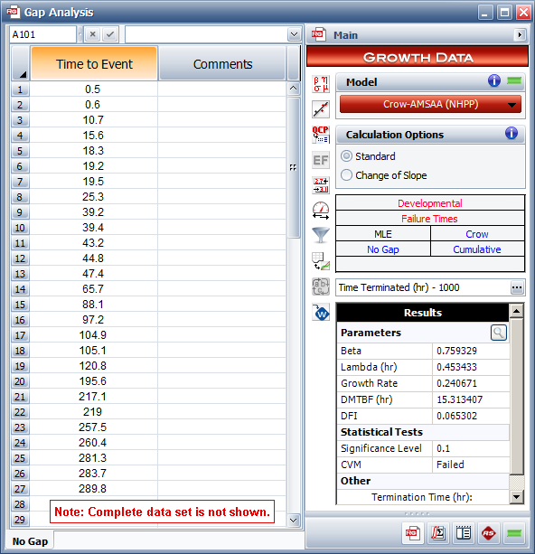
The results show that the data set failed the Cramér-von-Mises (CVM) goodness-of-fit test. This indicates that the model is not a good fit for the data.

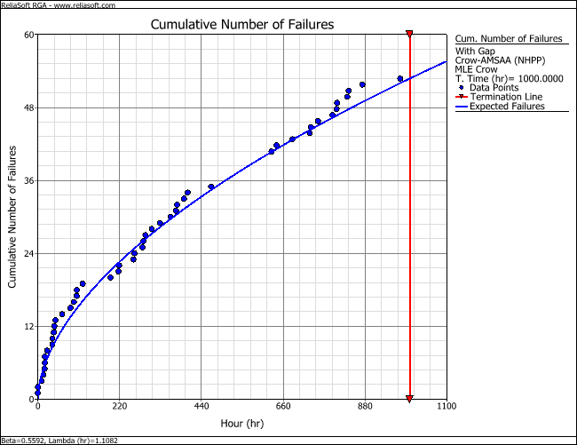
The following plot shows that the number of failures from 500 to 625 hours is abnormally high. A quick investigation found that new data collectors were assigned to the project at around that time and that extensive design changes involving the removal of several parts were also made within that period. It is possible that the parts that were removed were incorrectly reported as failed parts. Based on their knowledge of the system and the test program, the analysts agree that such a large number of failures were extremely unlikely. They decide to repeat the analysis using gap analysis.

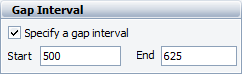
Return to the data sheet. On the Analysis page of the control panel, select the Specify a gap interval check box and then enter 500 to 625 for the gap interval, as shown next.

Return to the Main page of the control panel and analyze the data set by choosing Growth Data > Analysis > Calculate or by clicking the icon on the Main page of the control panel.

This time, the analysis will ignore the failure times observed between 500 and 625 hours. The resulting plot now shows that the model provides a much better fit to the data.

E-mail Link