Change of Slope Analysis

Change of Slope analysis can be applied to situations where a major change in the system design or operational environment causes a significant change in the failure intensity of the system. In this case, a single model may not provide a good fit for the data set.

To analyze this type of data set, the Change of Slope analysis splits the data set into two segments, based on the time that the change took place, and then applies a separate Crow-AMSAA (NHPP) model to each segment. The time that the change took place can be estimated from the data or based on your own knowledge about the specific change that was applied to the system. Note that although two separate models are applied to the segments, the information collected in the first segment are considered when creating the model for the second segment.

This analysis is available when you use the Crow-AMSAA (NHPP) model with any times-to-failure data type (except Multiple Systems with Event Codes) or with Discrete – Mixed data.

Note: The Change of Slope analysis requires at least three failures up to the break point and two failures after the break point (in the case of grouped data, this would be the number of intervals before and after the break point).

Example

The data set used in this example is available in the example database installed with the software (called "RGA19_Examples.rsgz19"). To access this database file, choose File > Help, click Open Examples Folder, then browse for the file in the RGA sub-folder.

A system is put through a reliability growth testing program. A total of 58 failures are observed during the 660 hours of testing. The data are recorded in a Failure Times data sheet and analyzed with the Crow-AMSAA (NHPP) model, as shown next.

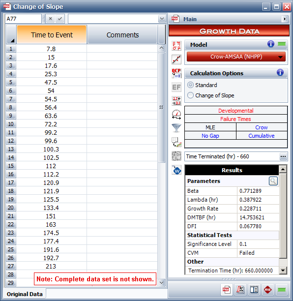
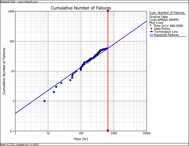
The results show that the data set failed the Cramér-von-Mises (CVM) goodness-of-fit test. This indicates that the model is not a good fit for the data. In addition, the following plot shows that there appears to be a significant change in the slope of the points at around 400 hours. As it turns out, a major design change was implemented at this point in time. Given this scenario, we can repeat the analysis using the Change of Slope methodology with the break point set to 400.

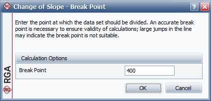
Return to the data sheet. In the Calculations Options area of the control panel, select the Change of Slope option, and then click the Calculate icon. This opens the Change of Slope - Break Point window, which allows you to specify the point at which the data set should be divided. Enter a value of 400, as shown next.

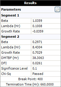
RGA automatically splits the data into two segments and fits a separate Crow-AMSAA (NHPP) model to each segment. For the first segment, the data points up to 400 hours are used to calculate its parameters. For the second segment, the data points after 400 hours plus information from the first segment are used to calculate its parameters.

The following results show the estimated parameters for Segment 2. Based on this model, the demonstrated MTBF (DMTBF) of the system at the end of the test is 38.3063 hours. (The Segment 1 model can be used to calculate the MTBF for times up to 400 hours only.) The results also show that the data set has passed the chi-squared goodness of fit test.

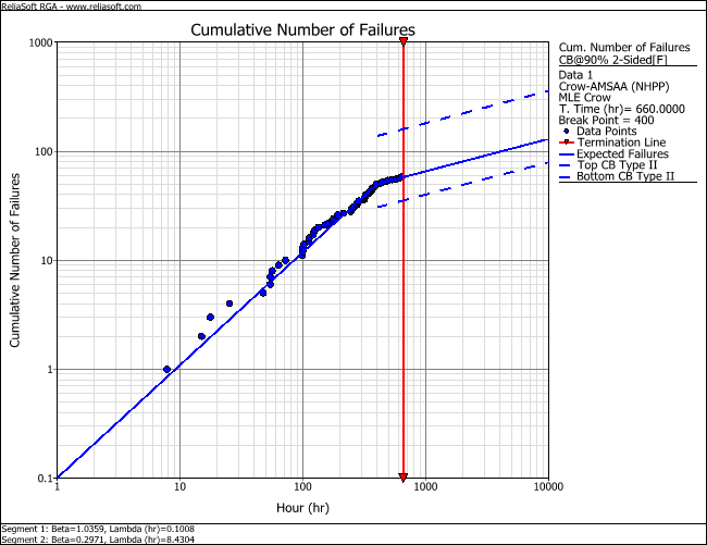
The following plot shows that the model provides a much better fit to the data. If you choose to display the confidence bounds on the plot, only the bounds on Segment 2 (which is the model of interest) will be plotted, as shown next.

E-mail Link