Related Topics and Links:
	Crow Extended Examples

Example Using the Crow Extended Model for Developmental Test Data

The name of the project is "Crow Extended - Failure Times," and the folio that contains the data is called "Corrective and Delayed Fixes."

Failure times for a single system undergoing developmental testing were recorded. Some of the observed failure modes were not addressed, some were addressed during the test and some were delayed until after the test. The test ended at 400 hours, and the goal is to estimate the following values:

• The MTBF demonstrated at the end of the test.

• The MTBF that can be expected after the BD failure modes are addressed.

• The maximum MTBF that can be achieved if all BD modes that exist in the system were discovered and fixed according to the current maintenance strategy (i.e., given the portion of the system's failure intensity that will be addressed by corrective actions).

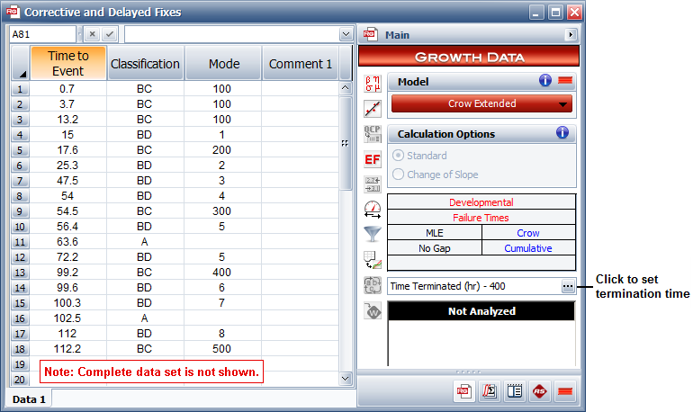
The data from the test are recorded in a Failure Times data sheet configured for cumulative failure times and with the Crow Extended model selected, as shown next. Modes classified as "A" are not addressed. "BC" modes are addressed during the test, and "BD" modes are addressed after the test. Numerical codes were used to identify the modes in the order in which they appeared (e.g., 100 and 200 are the first and second BC modes, 1 and 2 are the first and second BD modes, etc.). To specify that the test is time terminated at 400 hours, click the (...) button on the control panel to open the Termination Time window.

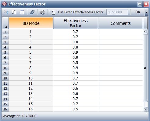
Next, enter an effectiveness factor for each BD mode to specify the effectiveness of each delayed fix (e.g., a factor of 0.7 means the fix will reduce the mode's failure intensity by 70%). To do this, choose Growth Data > Crow Extended > Effectiveness Factors or click the icon on the control panel.

Enter the factors shown next. You can see that the average effectiveness factor for all the delayed fixes—displayed in the status bar—is 0.7250. Click OK to save the changes and close the window.

Click the Calculate icon on the folio's control panel to analyze the data.

Note: This model uses the maximum likelihood estimation (MLE) method to calculate the parameters, which is known to produce a biased value for beta. This bias is more evident when working with small sample sizes. If the folio is not configured to remove this bias, you will be prompted to change the option in the Settings tab of the Item Properties window (Project > Current Item > Item Properties). To ensure the unbiased beta is always calculated for all new folios, use the Calculations page of the Application Setup window to select the option. This example assumes that the unbiased beta is calculated.

The results for all failure modes will appear as shown next.

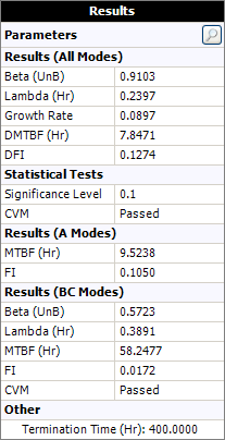
The beta, lambda and growth rate (1 - beta) parameters are shown in the table. In addition to these values, the table provides this information:

• The demonstrated/achieved mean time between failures (DMTBF/AMTBF) at the end of the test is 7.8471 hours.

• The demonstrated/achieved failure intensity (DFI/AFI) at the end of the test is 0.1274.

• The data is shown to have passed the Cramér-von Mises statistical test (CVM), which means we can accept the hypothesis that the failure times follow a non-homogeneous Poisson process (NHPP). This hypothesis is assumed by the Crow Extended model.

Next, to view all the desired values in a plot, click the Plot icon on the control panel.

Then choose Growth Potential MTBF from the Plot Type drop-down list. The plot appears as shown next.

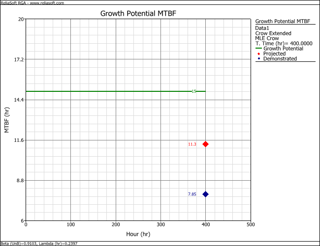
The following information is shown in the plot:

• The blue Demonstrated point shows the MTBF at the end of the test (before the BD failure modes are addressed) is 7.8471 hours.

• The red Projected point shows that, after the BD failure modes are addressed, the MTBF is expected to be 11.3182 hours.

• The green Growth Potential line shows that the maximum achievable MTBF given the current management strategy is 14.9957 hours.

© 1992-2019. HBM Prenscia Inc. ALL RIGHTS RESERVED.

E-mail Link