
The data set used in this example is available in the example database installed with the software (called "RGA11_Examples.rsgz11"). To access this database file, choose File > Help, click Open Examples Folder, then browse for the file in the RGA sub-folder.
The name of the project is "Repairable Systems - Race Car Analysis."
Failure times were recorded for three Formula 1 race cars operating in the field. Each car failed multiple times during the observation period. When a failure occurred, the failure time was recorded, along with the name of the failed component that was replaced. For example, the data set for the first car is shown next using the Advanced Systems View.
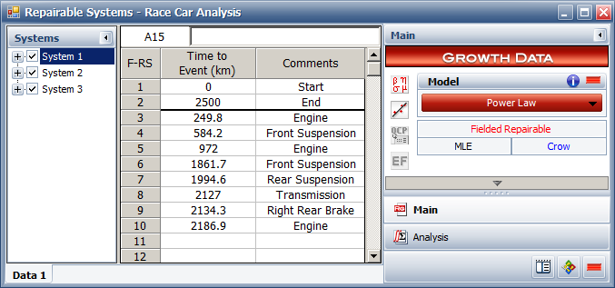
According to this data set, the first car was observed during its first 2,500 kilometers of operation. The engine was replaced when the car failed after 249.8 kilometers, the front suspension was replaced after 584.2 kilometers, and so on. Similar data sets are available for two others cars.
The goals of the analysis are to analyze the combined data from all three repairable systems in order to:
Estimate the total number of failures that you could expect for a car that competes in ten 200-kilometer races.
Determine the probability that a car that has finished two races will complete a third without any failures.
Determine if it would be feasible to overhaul the entire car at regular intervals in order to minimize its total life cycle cost. If it is feasible, calculate the overhaul time, assuming an average repair cost of $192,000 and an overhaul cost of $500,000.
On the control panel, choose the Power Law model, and then analyze the data by choosing Growth Data > Analysis > Calculate or by clicking the icon on the Main page.
![]()
A summary of the calculation results will then be shown on the control panel.
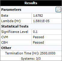
You can see in the results that the data passed the Cramér-von Mises (CVM) test, which indicates that the power law model provides a good fit for the data. (If the power law model did not provide a good fit, you could transfer the data to a Fleet data sheet and use the Crow-AMSAA model instead. The Fleet data sheet allows you to group the data and combine them into a cumulative timeline for analysis.)
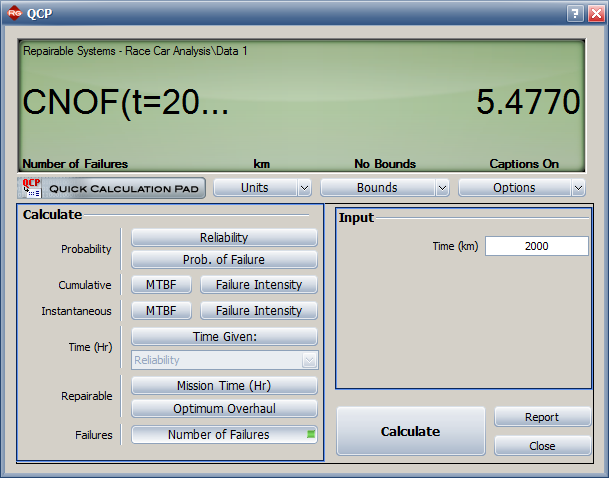
To estimate the total number of failures expected for one car over the period of ten 200-kilometer races, open the QCP by choosing Growth Data > Analysis > Quick Calculation Pad or by clicking the icon on the Main page of the control panel.
![]()
In the QCP, choose to calculate the Number of Failures with None for the confidence bounds. Select km for the time units and then enter 2000 (i.e., the equivalent of ten 200-kilometer races) in the Time field.
Click Calculate to obtain the result, as shown next. This analysis estimates about 5 failures for a car that competes in ten races.
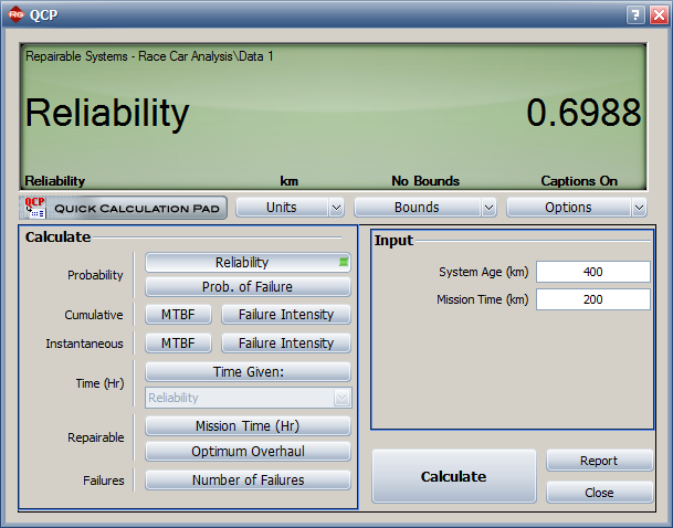
You can also use the QCP to determine the probability that a car that has finished two 200-kilometer races will complete a third race. Choose to calculate Reliability and make the following inputs:
System Age = 400 (i.e., two races, each 200 kilometers)
Mission Time = 200 (i.e., a third 200-kilometer race)
According to this result, the reliability of the car for the third race is estimated to be 69.88%.
Finally, to calculate an optimum overhaul time, first make sure the beta value of the fitted power law model is greater than 1 (indicating wearout). If the system has a constant failure rate (beta = 1) or a decreasing rate (beta < 1), then it will not be cost-effective to implement an overhaul policy.
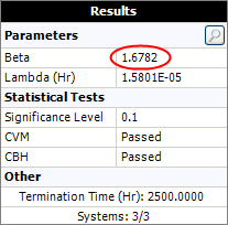
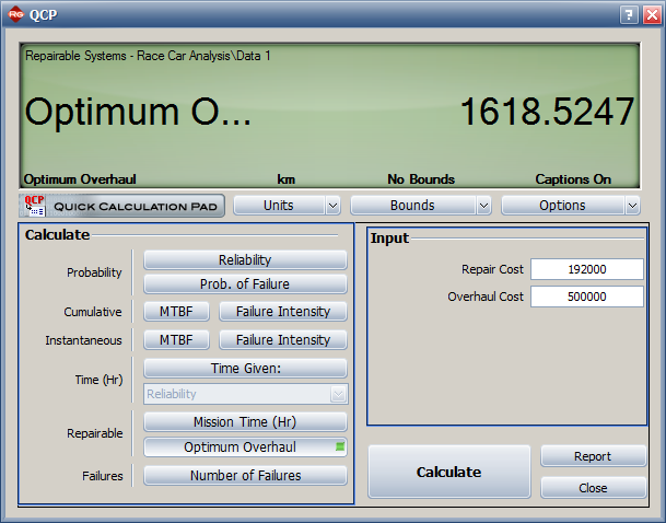
Since beta is greater than 1, you can use the QCP to solve for the optimum overhaul time. In the QCP, choose to calculate Optimum Overhaul, and then make the following inputs:
Repair Cost = 192000
Overhaul Cost = 500000
According to this result, the total life cycle cost of the car can be minimized by overhauling it every 1,619 kilometers.
© 1992-2017. HBM Prenscia Inc. ALL RIGHTS RESERVED.
 |
E-mail Link |