	Related Topics:
	Factorial Reliability Designs

Factorial Reliability Designs: Example

The data set used in this example is available in the example database installed with the software (called "doe9_examples.rsr9"). To access this database file, choose File > Help, click Open Examples Folder, then browse for the file in the DOE sub-folder.

The name of the example project is "Reliability DOE - Life Time Test of Fluorescent Lights."

In this example, two level factorial reliability DOE is used to determine the best factor settings to improve the reliability of fluorescent light bulbs. Five two-level factors were used in a fractional design to investigate the main effects of the factors and the interaction effect of the first two factors. It is assumed that none of the other interaction effects are significant and that the life of the bulb follows a lognormal distribution.

Each treatment in the design has two replicates (i.e., two bulbs were tested at each factor level combination), and the experiment was conducted over 20 days with inspections every two days. (The failure times were short because the lights were subjected to an accelerating factor that stressed the lights at higher than normal conditions.) Some of the units were still not failed at the end of the 20-day test.

Designing the Experiment

The design matrix and the response data are given in the "Fluorescent Light Life Test" folio. The following steps describe how to create this folio on your own.

Choose Insert > DOE > Add Standard Design to add a standard design folio to the current project.

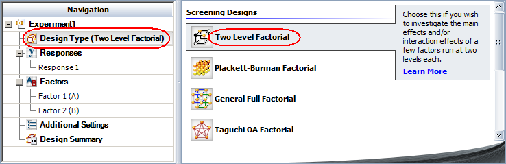
Click Design Type in the folio's navigation panel, and then select Two Level Factorial in the input panel.

Specify that you will be performing reliability DOE by clicking Response 1 in the navigation panel and choosing Life Data from the Response Type drop-down list. Then choose Both Suspensions and Intervals from the Censoring drop-down list to specify that some of the data points will be suspensions (i.e., times at which the unit was found not failed) and all of the times-to-failure data will be entered as intervals (since the units are inspected only once every two days).
Specify the number of factors by clicking the Factors heading in the navigation panel and choosing 5 from the Number of Factors drop-down list.
Define each factor by clicking it in the navigation panel and editing its properties in the input panel. In this example, the default labels are used for all the factors. (See Adding, Removing and Editing Factors.)
Rename the folio by clicking the Experiment1 heading in the navigation panel and entering Fluorescent Night Life Test for the Name in the input panel.
Click the Additional Settings heading to choose the number of replicates, specify the kind of fractional design that will be used and define the generators (i.e., aliased effects).
- Set the number of Replicates to 2 (since there are 2 units tested for each factor level combination).
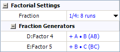
- Under the Factorial Settings heading, choose 1/4: 8 runs from the Fraction drop-down list. This means 8 runs will be used for each replicate of the design, instead of the 32 runs that would be required for a full factorial design.
- Since a fractional design is being used, you must choose Fraction Generators for the last two factors. Since it is assumed that the interaction effects AC and BC are not significant, you choose to alias the main effect of D with the interaction effect AC, and the main effect of E with the interaction effect BC, as shown next.

Finally, click the Build icon on the control panel to create a Data tab that allows you to view the test plan and enter response data.

Analysis and Results

The data set for this example is given in the "Fluorescent Light Life Test" folio of the example project. After you enter the data from the folio, you can perform the analysis by doing the following:

Note: To minimize the effect of unknown nuisance factors, the run order is randomly generated when you create the design in DOE++. Therefore, if you followed these steps to create your own folio, the order of runs on the Data tab may be different from that of the folio in the example file. This can lead to different results. To ensure that you get the very same results described next, show the Standard Order column in your folio, then click a cell in that column and choose Sheet > Sheet Actions > Sort > Sort Ascending. This will make the order of runs in your folio the same as that of the example file. Then copy the response data from the example file and paste it into the Data tab of your folio.

In the Distribution drop-down list on the Data tab control panel, select to use the Lognormal distribution for the analysis.
Make sure all main effects and the interaction effect AB will be considered. To do this, click the Select Terms icon on the control panel.

In the window that appears, select the Main Effects and A·B check boxes. Then click OK.

On the Analysis Settings page of the control panel, enter a Risk Level of 0.5 and choose to analyze Individual Terms.
Return to the Main page of the control panel and click the Calculate icon.

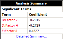
The results in the Analysis Summary area show that second, fourth and fifth factors have a significant effect on the bulb's life.

To see the coefficients for all the terms in the regression model, click the Detailed Summary link and view the MLE Information table.

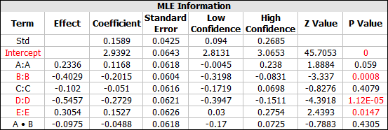
From the MLE Information table, you can see the model for the ln-mean or the scale parameter in the lognormal distribution is:

μ = 2.9392 + 0.1168A - 0.2015B - 0.051C - 0.2729D + 0.1527E - 0.0488AB

To view a plot comparing the standardized effect of each term, click the Plot icon.

Then choose Pareto Charts - Regression from the Plot Type drop-down list. The following plot appears.

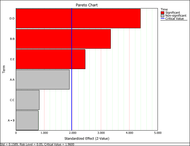
The horizontal blue line in the plot marks the critical value determined by the risk level specified on the Analysis Settings page of the control panel. If the bar goes past the blue line, then the effect is considered significant.

Conclusion

From the regression model, we can determine that in order to improve the reliability, factors B, C and D should be set to their low (-1) level, indicated by their negative coefficients, while A and E should be set at their high (+1) level, indicated by their positive coefficients. Under this setting, the predicted scale parameter in the lognormal distribution is 3.7829. Therefore, the life distribution under this factor setting is a lognormal distribution with a standard deviation of 0.1589 and ln-mean of 3.7829.

To do more advanced analysis, you can enter the data into ReliaSoft’s ALTA for accelerated life data analysis to further investigate the life stress relationship. Since factors A and C are not shown to be significant, they can be removed in further analysis.