Related Topics and Links:
	Crow Extended Examples Fielded Data

Example Using the Crow Extended Model for Operational Test Data

The name of the project is "Crow Extended - Operational Test Data for Two Systems," and the folio that contains the data is called "Operational Test Data."

Operational testing for two systems is performed towards the end of a new product development program. The systems are pilot builds and are subjected to representative customer use conditions during testing. When a system fails, a minimal repair is performed to bring the system back to operating condition (i.e., repairs are only enough to bring the system back to operation). Therefore, the configuration of each system during the test is assumed to not change and the reliability is assumed to neither deteriorate nor improve during the test (i.e., beta = 1). In addition, for each failure time, the associated failure mode is identified and classified.

The analysts have the following goals:

• Determine the MTBF that would be attained at the end of the basic reliability tasks if all the problem failure modes were uncovered in early design and corrected in accordance with the management strategy.

• Create a plot to determine whether new BD modes are being discovered at a decreasing rate throughout the test. If so, this would indicate that the number of remaining unseen BD modes is decreasing with time.

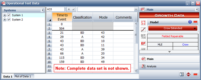
The data from the test are recorded in a Repairable data sheet with the Crow Extended model selected. Modes classified as "A" are not addressed, and "BD" modes are addressed after the test. Numerical codes were used to identify each specific failure mode. Some of the data for System 1 (selected in the Systems panel on the left) are shown next.

Before you can analyze the data, you must enter an effectiveness factor for each BD mode to specify the effectiveness of each corrective action that will be performed after the test (e.g., a factor of 0.7 means the corrective action will reduce the mode's failure intensity by 70%). To do this, choose Growth Data > Crow Extended > Effectiveness Factors or click the icon on the control panel.

In the window that appears, select the Use Fixed Effectiveness Factors option and then enter 0.6 in the input field. Click OK to save the factors and return to the folio.

Click the Calculate icon on the folio's control panel to analyze the data.

The results for all failure modes will appear as shown next.

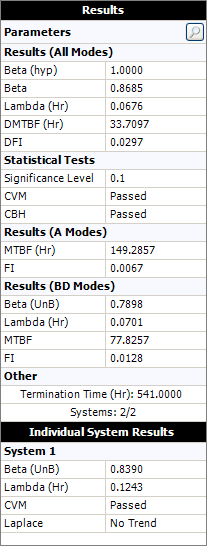
• The Parameters values include estimated parameters for the fitted model and other calculations based on those parameters.

• • The beta hypothesis, Beta (hyp), is the assumed beta value for the analysis. If this value is shown in red, then the beta = 1 assumption may not be valid.

  • The calculated Beta and Lambda parameters are 0.8685 and 0.0676. The calculated beta value is used to determine whether the beta = 1 assumption is valid. (If 0.8685 were significantly different from 1, then the assumption would be invalid.)

  • The demonstrated/achieved mean time between failures (DMTBF/AMTBF) at the end of the test is 33.7097 hours.

  • The demonstrated/achieved failure intensity (DFI/AFI) at the end of the test is 0.0297.

• The Statistical Tests values indicate whether the data meet various assumptions underlying the analysis.

• • The data is shown to have passed the Cramér-von Mises test (CVM), which means we can accept the hypothesis that the failure times follow a non-homogeneous Poisson process (NHPP).

  • The data also passed the Common Beta Hypothesis (CBH) test, which means the data sets from both systems can be assumed to have the same beta value.

To calculate the maximum attainable MTBF based on the current management strategy, click the Quick Calculation Pad icon on the control panel.

In the window that appears, select the MTBF option in the Projected area. After you click Calculate, the QCP will appear as shown next.

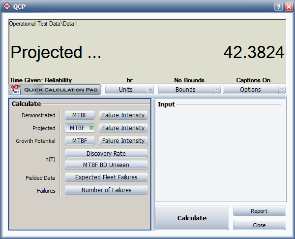
This result means the MTBF demonstrated at the end of the test (the DMTBF of 33.7097 shown on the control panel) is expected to increase to 42.3824 hours after all the BD modes have been fixed.

The next goal is to create a plot to examine how the failure intensity due to unseen BD modes changes over time. To do this, click the Plot icon on the control panel.

Then choose Discovery Rate from the Plot Type drop-down list and clear the Use Logarithmic Axes option on the control. The plot will appear as shown next.

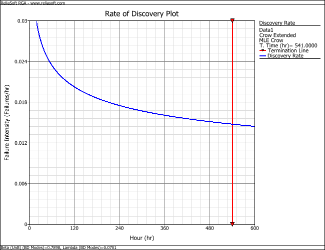
As unique BD modes are being discovered during the test, the unseen failure intensity decreases. This indicates that unique BD modes are being discovered at a decreasing rate, which is the desired outcome for a reliability growth test.

© 1992-2019. HBM Prenscia Inc. ALL RIGHTS RESERVED.

E-mail Link