
Discrete data are obtained from one-shot devices with only two possible outcomes from the test: success or failure. An example is a missile that gets fired once and it either succeeds or fails. This type of data is also referred to as success/failure or attribute data. Different data sheets are available depending on how the testing was conducted and what information is available. This also determines what kind of analysis can be performed.
With the first three discrete data types, you can use the Crow-AMSAA (NHPP), Standard Gompertz, Modified Gompertz, Lloyd-Lipow, Duane or Logistic models to track how the reliability of the system changes over time (traditional reliability growth analysis):
The fourth discrete data type can be used for either traditional reliability growth analysis or projections (growth projections analysis):
For the Mixed data type, if you will assume that all fixes are applied immediately after failure and before testing resumes (traditional reliability growth analysis), you can use the Crow-AMSAA (NHPP) model. If you want to account for different fix strategies used for different failure modes (growth projections analysis), choose the Crow Extended model.
When you select the Crow Extended model, the Classification and Mode columns will be inserted into the data sheet. You can also manually insert or remove these columns by choosing Growth Data > Format & View > [Insert Columns/Delete Columns] > Projections. The Crow Extended model and mode classifications are discussed in Failure Mode Classifications.
By default, all data sheets include a Comments column for logging any pertinent information about each row of data. You can add a second comments column or delete the columns by choosing Growth Data > Format & View > [Insert Columns/Delete Columns] > Comments. The information in these columns does not affect the calculations in the folio.
See also Minimum Data Requirements Discrete Data.
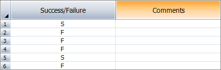
The Sequential data type is used for one-shot devices where a single trial is performed for each system configuration and improvements are made before the next trial. Only the outcome (success/failure) is recorded for each trial.
The device is inspected after each trial, and then fixes are applied before the next trial begins; therefore, each row number in the data sheet represents a particular design configuration. In the following example, the device succeeded (S) for the first configuration (row 1), but failed (F) for the second configuration (row 2). The rest of the data can be read in a similar manner.
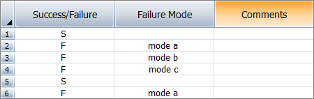
The Sequential with Mode data type is used for one-shot devices where a single trial is performed for each system configuration and improvements are made before the next trial occurs. In addition to the outcome (success/failure) for each trial, the specific failure modes are also recorded.
The data sheet is the same as the Sequential data sheet, but with the addition of a Failure Mode column for recording the mode responsible for each failure. This allows you to track the possible recurrence of a failure mode after the fixes have been applied. If the mode does not appear again in the later trials, then the probability of failure is reduced. This is known as failure discounting. If you do not enter any failure modes, then no failures are discounted in the analysis (and the results will be the same as in the Sequential data type if you use the same growth model). The following figure shows an example of the data sheet.
The Grouped per Configuration data type is used for one-shot devices where multiple trials are performed for each design configuration (e.g., testing 5 missiles of the same design equals 5 trials). Improvements are made after all the devices within the group have been tested. Therefore, each row in the data sheet represents a particular design configuration. For each stage of testing, both the number of trials and the number of failures are recorded (e.g., 3 failures out of 10 trials for configuration A, 2 failures out of 10 trials for configuration B, etc.).
The Number of Trials column is for recording the number of devices that were tested for each design configuration. The Number of Failures column is for recording the number of failed units in the specified configuration. The values in these columns can be cumulative (where each row shows the total number of trials and failures since the beginning of the test) or non-cumulative (where each row shows the incremental number of trials and failures from the last configuration). (See Cumulative vs. Non-Cumulative Data.)
The following example shows a data set where the values are cumulative. In the first configuration (row 1), there were 5 failures out of 10 trials. In the second configuration (row 2), there were 3 more failures (for a total of 8) out of 8 more trials (for a total of 18). The rest of the data can be read in a similar manner.
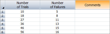
Grouped per Configuration Data Sheet (Cumulative)
The next example shows the same data set, but the values are non-cumulative.
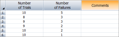
Grouped per Configuration Data Sheet (Non-Cumulative)
The Mixed data type is used for one-shot devices where some test stages (i.e., design configurations) may have only one trial while other stages may have multiple trials. For each stage of testing, both the number of trials and the number of failures are recorded (e.g., 1 failure out of 1 trial for configuration A, 2 failures out of 5 trials for configuration B, etc.). This data type may be used in cases when you have a different number of samples available from each design configuration. For example, you might test one device initially then later start testing more samples of each design.
The Failures in Interval column is for recording the number of failures in a stage. The Cumulative Trials column is for recording the total number of trials that were performed since the beginning of the test.
When you use the Crow-AMSAA (NHPP) model for this data type, the assumption is that fixes are applied at the end of each interval; therefore, each row in the data sheet will represent a different design configuration, where each configuration can have any number of trials. For example, the following data set shows that in the first stage (row 1), 4 units were tested and 3 failed. In the second stage (row 2), 1 more unit was tested (for a total of 5) and it did not fail. In the third stage (row 3), 4 more units were tested (for a total of 9) and all 4 failed. The rest of the data can be read in a similar manner.
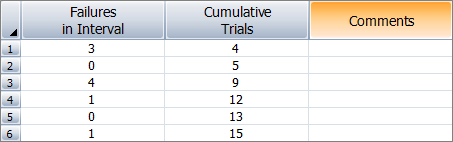
Mixed Data Sheet with the Crow-AMSAA (NHPP) Model
When you use the Crow Extended model, you assume that some of the fixes may be delayed until the end of the test and that some of the failure modes may not be fixed (i.e., A = no fix or BD = delayed fix). This is useful for situations when you need to perform the test in stages due to logistic reasons (e.g., cannot launch 10 missiles at the same time), or the purpose of the test is only to uncover failure modes. You will be required to identify and classify the failure mode responsible for each failure, and specify the effectiveness factor for each delayed fix, if any (see Failure Mode Classifications).
For example, the following data set shows that in the first stage (rows 1 to 3), 4 units were tested and 3 failed. The failures are identified as BD125 (row 1), A10 (row 2) and BC230 (row 3). In the second stage (row 4), 1 more unit was tested (for a total of 5) and it did not fail. The rest of the data can be read in a similar manner.
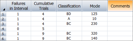
Mixed Data Sheet with the Crow-Extended Model
Tip: If you will assume that some fixes are implemented at the end of an interval while some are implemented at the end of the observed test time, then the Multi-Phase Mixed data type may be more appropriate.
© 1992-2019. HBM Prenscia Inc. ALL RIGHTS RESERVED.
| E-mail Link |