Example: Failure Times Data

The data set used in this example is available in the example database installed with the software (called "RGA11_Examples.rsgz11"). To access this database file, choose File > Help, click Open Examples Folder, then browse for the file in the RGA sub-folder.

The name of the project is "Failure Times - Duane and Crow-AMSAA," and the folio that contains the data is called "Crow-AMSAA (NHPP)."

A prototype of a system is tested at the end of one of its design stages. When a failure occurs in the system, the time of failure is recorded and then a fix is applied before testing resumes. A total of 40 failures were observed during this period. The prototype has a design specification of an MTBF = 135 hours with a 90% confidence level. The goal is to determine whether the prototype meets the specified MTBF goal.

The data from the test are recorded in a Failure Times data sheet configured for cumulative failure times, as shown next. To specify the time when the test ended, click the (...) button on the control panel to open the Termination Time window. Select Failure Terminated and click OK.

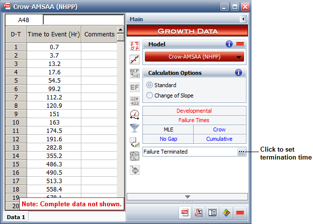
On the control panel, choose the Crow-AMSAA (NHPP) model, and then analyze the data by choosing Growth Data > Analysis > Calculate or by clicking the icon on the Main page of the control panel.

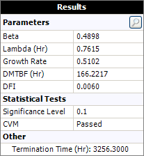
The results show a demonstrated MTBF (DMTBF) = 166.2217 hours at the end of the test, as shown next.

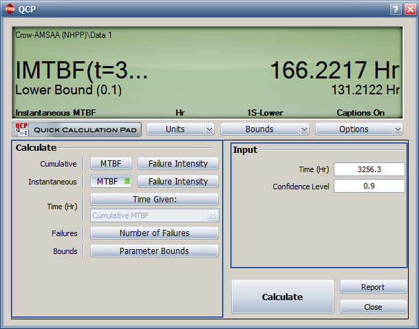
You can use the Quick Calculation Pad (QCP) to obtain the 90% confidence bounds on the demonstrated MTBF. To access the QCP, choose Growth Data > Analysis > Quick Calculation Pad or click the icon on the Main page of the control panel.

In the QCP, select to calculate the instantaneous MTBF with lower one-sided confidence bounds. Select Hour for the time units and then make the following inputs:

Click Calculate to obtain the results. It shows that the lower limit on the MTBF at the specified time with a 90% confidence level is 131.2122 hours. Therefore, the prototype has met the specified goal.

To create a plot of the result, close the QCP, and then choose Growth Data > Analysis > Plot or click the icon on the Main page of the control panel.

On the plot's control panel, click the Plot Type drop-down list and choose MTBF vs. Time. The following plot shows the cumulative MTBF and the corresponding instantaneous MTBF on a logarithmic plot. (Note that you can switch to a linear scale by clearing the Use Logarithmic Axes check box on the plot's control panel).

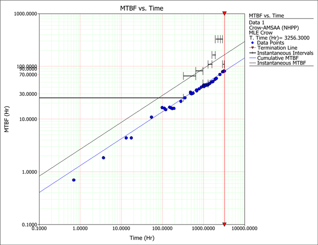
The points represent the actual failure times in the data set, while the vertical line represents the test termination time. The horizontal lines on the plot are the instantaneous intervals, which show the MTBF over a specified interval length. The MTBF over an interval is obtained by dividing the length of the interval with the number of failures in that interval. The intervals can be used to observe a general MTBF trend, whether the MTBF increases, decreases or stays the same over time.

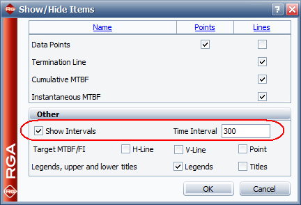
You can specify the length of the intervals by choosing Plot > Actions > Show/Hide Items or by right-clicking the plot and choosing Show/Hide Items on the shortcut menu.

In the window, make sure that the Show Intervals check box is selected, and then specify the length of the interval in the Time Interval field, as shown next. Click OK and the plot will refresh to show the new results.

E-mail Link