Related Topics:
	Multiple Linear Regression Folio

Multiple Linear Regression Folio: Example

The name of the example project is "Multiple Linear Regression - Ice Cream Consumption."

The multiple linear regression folio provides an easy way to quickly analyze existing data. In this example, ice cream consumption per capita was measured in four-week periods from March 18, 1951 to July 11, 1953 in order to determine whether it depended on the price of ice cream, the weekly family income and/or the mean temperature.

Creating the Folio

To investigate the predictors, the analysts use DOE++ to create a multiple linear regression folio. Then they enter the predictor and response values on the Data tab. The design matrix and the response data are given in the "Ice Cream Consumption" folio. The following steps describe how to create this folio on your own.

• Choose Insert > Tools > Add Multiple Linear Regression to add a new folio to the current project.

• Double-click the column headers to rename each of the columns.

• Click the arrow inside a header to specify whether the column contains predictor data (e.g., mean temperature) or response data (i.e., ice cream consumption).

Analysis and Results

The data set for this example is given in the "Ice Cream Consumption" folio of the example project. After you enter the data from the example folio, you can perform the analysis by clicking the Calculate icon.

The ANOVA table and the Regression Information table for the model are available in the Analysis Summary window after you click the Detailed Summary link on the control panel. The R-sq and R-sq(adj) values in the ANOVA table indicate that the model fits the data relatively well.

The Regression Information table indicates that weekly family income and mean temperature are good predictors for ice cream production.

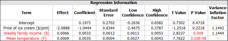
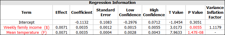
Since the price of ice cream does not seem to predict ice cream consumption, the folio was duplicated in the "Reduced Model" folio, where the price column was removed from the analysis by clicking the arrow in the header and clearing all the check boxes. Click the Detailed Summary link in the new folio to view the final regression model.

Click the Plot icon to view the residual vs. order plot, which you can use to look for outliers in the data set.

Conclusions

Based on the analysis, weekly family income and mean temperature are found to be the most significant factors in ice cream consumption. From the residual vs. order plot, we see that there are a few outliers but the majority of our data set fits the model. Thus, if desired, we could use the Prediction window to predict future ice cream consumption based on different combinations of family income and mean temperature.